Home Science Page Data Stream Momentum Directionals Root Beings The Experiment
In this section we will seek to show that each derivative of the Data Stream, directional or deviational, can be written solely as a function of the raw Data.
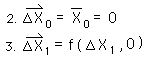
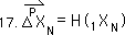
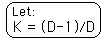
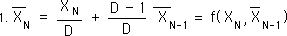
We start with the definitional equation for the Decaying Average. It is written as a function of one piece of Data and the previous average.
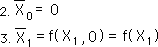
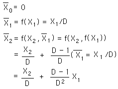
For a continuous Data Stream, all the initial derivatives equal zero. {See Deviation Notebook.} Because of this, the first Decaying Average is only a function of X1, the first Data Point.
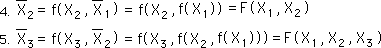
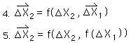
The 2nd Average is a function, f, of the 2nd Data Point and the 1st Average. The 1st Average is a function of the first Data Point only. So the 2nd Average is a new function, F, of the first and 2nd Data points. In a similar fashion the 3rd Average is a function, F, of the first three Data Points.
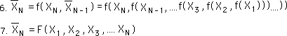
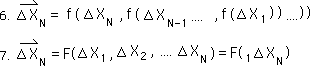
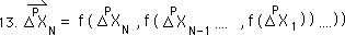
Finally, using the same logic, the Nth Average is a function, F, of the first N Data Points. F is a function, based upon nested f functions, the Decaying Average function.
For notational simplicity, the following equation represents the same thing as the preceding equation, just with different notation.
In a similar fashion we can show that the First Directional is also a function of all the raw data points.
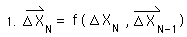
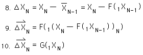
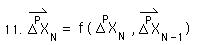
The first Directional is a decaying average of the decaying average. Thus it is a function of the change and the previous first directional, as we defined it in the Derivative Notebook.
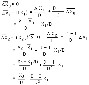
All the initial directionals equal zero. Thus the First Directional of the first Data point is a function of the First Change only.
Reasoning in a similar fashion we see that the First Directional of the second point is a function of the first two changes.
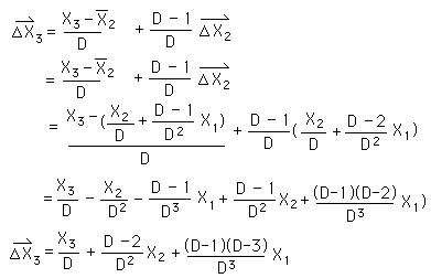
It is easy to see that the first Directional of the Nth Data point would be a function of all the N changes. It would be the same function, F, of nested f functions, that we referred to above in defining the Decaying Average, the initial Derivative.
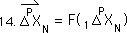
The Nth change is defined as the difference between the Nth data Point, XN, and the previous average. We substitute functions for the Decaying Average and find that the Nth point of the first directional would be a new function, G, of all the first N Data Points.
With similar logical steps, we can show that the Nth point of the Pth Directional is a grander function, H, of the first N Data Points. The H function consists of nested functions of nested functions, and so on, to nested G functions, nested F functions, back to the original nested f function, the Decaying Average function. The Nth point of the Pth Directional would be a function of the Nth point of the Pth level of change and the previous Pth Directional.
The initial Pth Directional is zero as always.
Using the same reasoning as above, the Pth Directional becomes a function, F, of all N of the Pth Level of Changes.
The F function is the same functions of nested f functions described above.
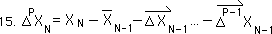
The Pth level of change is the difference between the raw data and all the previous directionals.
Each of these Directionals can be written as functions of all the raw Data except the most recent, XN, which is Raw Data.
Therefore a function, H, exists that will define the Pth Directional in terms of all N of the Data Points only.
This reasoning can also be applied to Deviations also, so that the Pth Deviational can be written as a function of just the raw data points.
So why waste time with these in-between stages? Why not write the derivatives as a function the raw data? Why worry about all of the lesser deviations or directionals? Why not just go to the heart of the matter, the raw Data, to define our higher directionals and deviations? Why define our Derivatives by their context when we can go right to the content, the raw Data, to define them instead. Let's go that route and see what happens.
Let us break some of the Derivatives into their elemental parts. Let us write them in terms of the nested f functions.
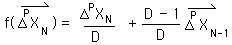
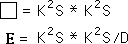
Below are the formula for the Decaying Average, the general expression for f function for Deviations, and the f function for Directionals.
Using these formulas, we find an expression for the 1st and 2nd point of the Decaying Average.
After some initial simplicity with the first Average, the second Average is already getting a bit complex.
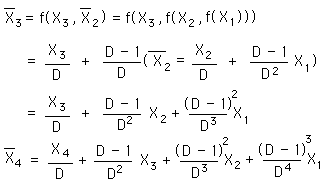
Using the same method, we derive the 3rd & 4th points of the Decaying Average. We see a pattern, complex not simple.
Now we are ready to look at the generalized F function, the function that defines our Decaying Average only in terms of the Raw Data.
First a notational simplification.
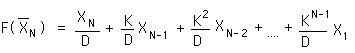
The above F function is written in terms of the nested f functions, the Decaying Average function.
In a simplification, multiplying through the Ks we arrive at the above equation. This is the F function for the Decaying Average. The Decaying Average is defined only by the raw data. A simplified expression? Not really.
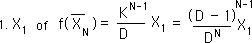
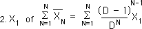
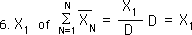
We can pick out the first Data Point’s contribution to the Nth Decaying Average from the last equation for the F function above. The greater N becomes, the smaller X1's contribution to the average of XN.
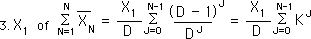
The contribution of X1 to all the averages up to the average at XN would equal to the following.
This is a power series that can be written more simply as:
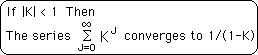
A common calculus theorem states that:
K is less than 1 because D-1 is less than D. So our power series converges to 1/(1-K). With a little algebra our proof is complete.
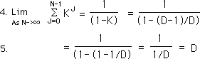
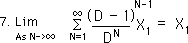
Replacing the sum with its limit in the equation for X1's contribution to the Decaying Average Stream, we get:
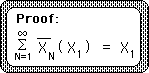
Our proof is complete and stated below.
So X1's contribution to the Decaying Average Stream approaches X1 as N, the number of elements in the Data Stream becomes larger and larger. The implication is that each piece of Data comes in diminished but is fully used up eventually – by the time the Data Stream reaches infinity (in non-mathematical terms.) As an example: If our Data Stream represented monthly savings, then as long as the sum of the areas of the Decaying Averages graph was greater than zero, there would still be some money left.
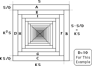
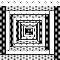
The above result will now be demonstrated visually.
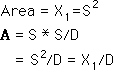
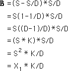
The area for the whole square is X1. If we partition off a Dth of this square, then its area is X1/D, which is section A. In this example D = 10.
For section B we leave the width the same but reduce the length by S/D, which is the width. This is the same as multiplying A’s area by K, which equals (D-1)/D. See above. B’s area equals X1*K/D. This is the same contribution that X1 makes to the average associated with X2.
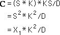
For section C we leave the length the same but multiply the width by K. This is the same as multiplying B’s area by K. C’s area equals X1*K2/D. This is the same contribution that X1 contributes to the average associated with X3.
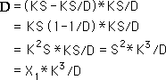
For section D we leave the width the same. The length is confined by the square. After the algebraic simplification D’s area equals X1*K3/D. This is the same contribution that X1 contributes to the average associated with X4.
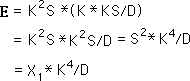
D’s width is the same as C’s width. B’s width is the same as A’s width. D’s length equals A’s width and C’s width subtracted from the whole side, S. E’s length equals B’s width & D’s width subtracted from the whole side, S. Therefore section E has the same length as Section D. We multiply E’s width by K. After algebraic simplification E’s Areas equals X1*K3/D. This is the e same contribution that X1 contributes to the average associated with X5.
Section E is inside the top of a rectangle, where its length is the top of the rectangle. Section D is outside the rectangle, but its length is the side of the rectangle. Because E’s and D’s length are equal, this interior rectangle is a square. Furthermore its side equals K2*S. Hence E’s width is a Dth of the width of the interior square. So E’s relation to the interior square is the same as A’s relation to the exterior square. We continue this process ever inward. Next. F’s width is kept constant while its length is shortened by 1/D. This has the effect of multiplying the previous area by K. Then G’s length is kept constant while its width is shortened by 1/D, Then H’s width is kept constant while its length is shortened by 1/D. This process continues ever inward.
This spiral graph represents X1’s decay, but it also represents the potential impact of each Data Piece on the Decaying Average. Section A would represent the Potential Impact of XN upon the Decaying Average. Section B would represent the Potential Impact of XN-1 upon the Decaying Average. Section C would represent the Potential Impact of XN-2 upon the Decaying Average. It is easy to visually perceive that, while each Data Point continues to exert some influence upon the average, the potential impact shrinks substantially over time.
Again the first point of the first Directional is a snap, simplicity. However the second point is already becoming a bit complex.
This point cures us of any hope for simplicity. The contribution of each of the Data Points to this first Directional becomes more and more complex.
We could probably derive some type of expression for X3, X2 and X1's contribution to the general point of the first Directional, but it's not going to be simple and has no immediate interest. This is a low level application of the simple G function. Remember that the G function writes the first directional in terms of the Data only.
No caveman would even attempt this type of calculation, consciously or subconsciously. First there are so many facts to remember. Second the patterns are so different for each directional that subconsciously memorizing them would never accidentally occur. But why do we care about a caveman's simplicity when we have our modern computers? We are trying to make a straightforward case for evolution. The simpler the mechanism the easier it is passed on. Complicated formulas and subtle approximation techniques with lengthy iterations are great for high speed computers but don't provide a competitive advantage to the evolving organism.